
RedisGraph and Redis: What, Why, and How
Learn More

A knowledge graph can be a simple data structure that represents what we know about part of the real world. For example, imagine searching for a product on your favorite shopping site. You might search for “glitter shoelaces” and expect to see whatever shoe-lacing products that match that specific term.
But how does the site know to display other shoe parts, or shoes themselves? The simple answer would be products that match a single term (e.g., “shoe”). But as people with knowledge of the world around us, we know a lot about this particular search choice that can help provide better responses.
This blog post explores how knowledge graphs work, how they’re used in computing, and how to use them with Redis Enterprise’s RedisGraph module. We’ll explore briefly how you can use Cypher queries to access information in a knowledge graph. Finally, we’ll talk about working with knowledge graphs at scale and discuss their future uses. If you’re interested in building a knowledge graph to enhance your machine learning applications, this is a great place to start.
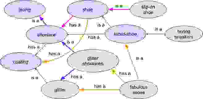
The search term is a particular kind of product—a shoelace with a coating—that we can represent in an ontology of objects in a knowledge graph. While there might appear to be a lot of things going on in the graph above, I’ve simplified it into two kinds of relations: “is a” (a category subtype) and “has a” (a part of something). For example, a shoelace is a lacing, a part of a shoe, and has a coating, or a laced shoe has a shoelace. The algorithm has no a priori knowledge of the world aside from what we’ve encoded in the graph.
When a user searches for “glitter shoelaces,” a search algorithm can identify a direct match in the ontology. With the knowledge graph, the algorithm can now understand that such an item has a glitter coating and is part of a larger category of items called “shoelaces” or even “lacing” (the purple arrows). It also can follow the “has a” relationship with “shoe” to understand that it is part of a larger item in the product catalog.
When we market products, we have choices as to what we can do with the relationships. While the simple choice is to display various categories of shoelaces, maybe we want to show an anti-pattern: shoes with no laces! We can follow the “has a” path back to shoes and query the graph for products that have no shoelace part (the magenta arrows) and display that as an alternative result.
Similarly, perhaps the consumer is trying to replace broken laces and we’d be better off showing them new shoes that match their preferences. In our ontology, shoes have coatings as well (the orange arrows) and we can find products that have both glitter shoelaces and a glitter coating (also in orange). Maybe they’d prefer a fabulous new shoe over replacing those broken glitter shoelaces?
While the technique of using graph data structures has been around in computing for a long time, the term “knowledge graph” was popularized by Google in 2012. The use of a graph as basis for representing knowledge has a long history, from the early days of the Web with RDF (1997) to now, where it’s often used in various areas of machine learning (ML), natural language processing (NLP), and search.
Knowledge graphs are often conceptualized as a way to capture what we know about a particular domain. The graph represents the terms, relationships, and instances of facts and concepts. What we know is represented as data that can be processed by algorithms, rather than algorithms that encode knowledge as rules written in code.
This representation of knowledge as data in a graph is an important distinction that makes using knowledge graphs important to search and model inference in machine learning. What we can understand about the world can be encoded and changed over time as we learn, without necessarily rewriting all our software components. In turn, models can learn by being re-trained continuously on the information encoded in the knowledge graphs. This cycle has become increasingly important for applications where the scale of data is massive and ever increasing.
Redis Enterprise’s RedisGraph module can help load and use ontologies when building knowledge graph infrastructures. The ontology’s structure becomes a set of graph nodes and edges with labels that can be queried via Cypher and searched via RediSearch. A simple ontology use case—such as looking up a referenced term and using the relationships in the graph to follow graph edges to find synonyms, superclasses, or other related terms—can be as simple as a single Cypher query.
For biology/biomedical domains, for example, there are community-developed ontologies available at the Open Biological and Biomedical Ontology (OBO) Foundry. The ontologies are available in the OBO and OWL formats and cover a variety of domains. Given the current pandemic, let’s look at the Coronavirus Infectious Disease Ontology.
There is also a Python library, called pygobo, that I developed for reading and transforming the OBO ontologies into a property graph that can be used with RedisGraph. The Coronavirus Infectious Disease Ontology is distributed in OWL format and so, once we convert it into OBO format, we can load the ontology and take a look at its structure.
Let’s take a look at this ontology by starting a local RedisGraph instance:
% docker run -p 6379:6379 redis/redisgraph
We can then load the ontology, here locally called “cido.obo”:
% pip install pygobo

% python -m pygobo load cido.obo --graph cido
With this completed, the ontology has been loaded into a graph called “cido.” The structure of this graph is documented on GitHub, but here’s a simple summary: There are nodes labeled Ontology and Term, ontologies have a “term” relationship, and terms relate to terms with a “is_a” relationship. For example, we can query for the term “antiviral drug” with:
MATCH (r:Term) WHERE r.name='antiviral drug' RETURN r
A more interesting query would be to retrieve the whole hierarchy of terms related to antiviral drugs that are within a certain depth of the “is_a” relationship.
MATCH (r:Term) WHERE r.name='antiviral drug'

MATCH p=(:Ontology)-[:term]->(:Term)<-[:is_a*1..3]-(r)

RETURN p
The RedisInsight visualization below shows the relationships of all the paths returned in this query. In the right bottom of the image is the “antiviral drug” node that we chose as a root. In the middle is the ontology node. The yellow arrows between nodes show the “is_a” relationship between the terms. Finally, the gray arrows show the term relationship between the ontology node and the term nodes.
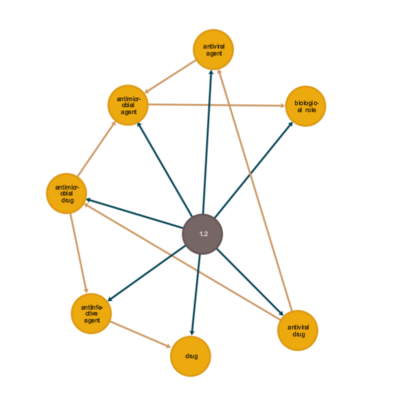
In the visualization, we can follow “is a” relationships from the “antiviral drug” node in the right corner to “antiviral agent” and “antimicrobial drug.” These both lead to “antimicrobial agent.” This subgraph retrieved by a simple query gives us an expanding set of categories and an understanding of the “is a” relationship. If we would like to search for alternative treatment for a particular drug, traversing these relationships allows us to discover a larger category or an alternative category.
Note that the ontology itself does not have instance data. That is, there are no drugs with the label “antiviral drug.” If we want to use this ontology with a database of drugs, we would simply include the identifier of the term node (i.e., the “id” property), which is guaranteed to be a unique value. Then queries can be used to navigate from a result in the drug database into the ontology.
For example, if a drug database is tagged with “CHEBI:36044” (antiviral drug), this simple query will discover the superclass terms “CHEBI:22587” (antiviral agent) and “CHEBI:36043” (antimicrobial drug):
MATCH (r:Term) WHERE r.id='CHEBI:36044'

MATCH (t:Term)<-[:is_a]-(r)

RETURN t.name,t.id
These terms can be used as additional search parameters that can expand the search results from the drug database. While very simple, this kind of ontological reasoning allows the database search algorithms to be independent of the term organization.
Knowledge graphs are an essential information resource for various scalable applications of machine learning in search and inferencing, as we’ve shown with retail and medical examples. A knowledge graph can be used to extend the hand-curated aspects of an ontology into the instances of data that relate to items within the ontology. Instances of data are often annotated, by hand or automatically by algorithms, with terms from the ontologies.
For example, the Gene Ontology has been used to annotate articles in PubMed so that search algorithms can apply logical reasoning to the ontology terms about gene function. The labeling of abstracts within PubMed with ontology terms extends the classifications from the ontology into metadata about the articles. Yet, this was initially largely done by human annotation and curation of labels.
The result of extending the ontology into instance data is what makes the result a knowledge graph—it includes both the data and information about the data in one large graph. The challenge here is to do this kind of analysis at scale. Human curation of annotation of data, while very important in some cases, will not scale to the vast amounts of data now being created.
When processing a large amount of data, inferencing via machine learning, text analysis via natural language processing, and harvesting data off the Web via human-curated information annotations (i.e., schema.org annotations) all allow a wide variety of data to be stored and categorized in a knowledge graph. The large scale of the data processed enables algorithms to navigate from a particular instance to a very large set of similar items by traversing from the instance data in the graph through the ontology terms to another set of related data. The terms and relations in the ontology allow us to know something about how two specific items relate to each other as part of a very large set of information.
The critical point here for scalability is that the ontology part of the knowledge graph is much smaller than the instance data. We can easily store the ontologies in RedisGraph, either as a single graph or multiple graphs, and use the other data structures within Redis or elsewhere to store instance data. It is not necessary to use graph-based representations for instance data, which may already be tabular.
From these building blocks we can build algorithms for search, provide recommendations to users of a service, or provide ways for experts to summarize and follow relationships within large amounts of information. Careful construction of the knowledge graph lets systems support professionals (e.g., in clinical settings or for drug development) where the classification of information is important to the correct outcome.
The scale of instance data may be too large to practically store in a graph structure. Fortunately, knowledge graphs do not have to be completely realized as graphs. For example, instance data can be stored in a scalable tabular data store where it can be easily augmented with term annotations. In particular, the tabular data can also be stored in Redis alongside the related ontologies stored via RedisGraph.
A query result from the tabular data with term annotations can be used by algorithms to find matching terms in the ontology. As we saw previously, the matches in the ontology form a subgraph of information. We can use this subgraph as model inference input. Subsequently, the output of the model inference can be used directly or for additional queries. The composition of the various queries and inference creates a powerful and flexible system with atomic query properties.
We can also query the ontology using the RediSearch features of RedisGraph to perform full-text searches of term names, descriptions, and relations. Once candidate terms are identified, we can use the same techniques with the subgraph from the ontology as a mechanism to query data previously stored in Redis. For example, we can find a tabular row annotated with one of the matching terms from the full-text search. The ontology provides us a domain-specific way to filter search results.
The techniques discussed here all use a single ontology. RedisGraph can store multiple ontologies and other graph structures in a single larger graph or as separate graphs under separate keys. This flexibility allows algorithms to be created by combinations of different graph components in a larger data pipeline.
The possibilities for implementing and using knowledge graphs within Redis are widespread. You can try out ontologies and knowledge graphs on RedisGraph via Docker, with Redis Enterprise, or on our Redis Cloud Pro service.