
This post is part five of a series of posts examining the features of the Redis-ML module. The first post in the series can be found here. The sample code included in this post requires several Python libraries and a Redis instance with the Redis-ML module loaded. Detailed setup instructions for the runtime environment are provided in both part one and part two of the series.
Decision Trees
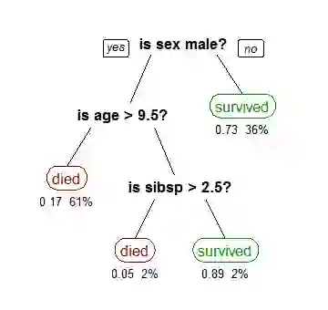
Decision trees are a predictive model used for classification and regression problems in machine learning. Decision trees model a sequence of rules as a binary tree. The interior nodes of the tree represent a split or a rule and the leaves represent a classification or value.
Each rule in the tree operates on a single feature of the data set. If the condition of the rule is met, move to the left child; otherwise move to the right. For a categorical feature (enumerations), the test the rule uses is membership in a particular category.
For features with continuous values the test is “less than” or “equal to.” To evaluate a data point, start at the root note and traverse the tree by evaluating the rules in the interior node, until a leaf node is reached. The leaf node is labeled with the decision to return. An example decision tree is shown below:
Many different algorithms (recursive partitioning, top-down induction, etc.) can be used to build a decision tree, but the evaluation procedure is always the same. To improve the accuracy of decision trees, they are often aggregated into random forests which use multiple trees to classify a datapoint and take the majority decision across the trees as a final classification.
To demonstrate how decision trees work and how a decision tree can be represented in Redis, we will build a Titanic survival predictor using the scikit-learn Python package and Redis.
Titanic Dataset
On April 15, 1912, the Titanic sank in the North Atlantic Ocean after colliding with an iceberg. More than 1500 passengers died as a result of the collision, making it one of the most deadly commercial maritime disasters in modern history. While there was some element of luck in surviving the disaster, looking at the data shows biases that made some groups of passengers more likely to survive than others.
The Titanic Dataset, a copy of which is available here, is a classic dataset used in machine learning. The copy of the dataset, from the Vanderbilt archives, which we used for this post contains records for 1309 of the passengers on the Titanic. The records consist of 14 different fields: passenger class, survived, name, sex, age, number of siblings/spouses, number of parents/children aboard, ticket number, fare, cabin, port of embarkation, life boat, body number and destination.
A cursory scan of our data in Excel shows lots of missing data in our dataset. The missing fields will impact our results, so we need to do some cleanup on our data before building our decision tree. We will use the pandas library to preprocess our data. You can install the pandas library using pip, the Python package manager:
pip install pandas
or your prefered package manager.
Using pandas, we can get a quick breakdown of the count of values for each of the record classes in our data:
pclass       1309
survived     1309
name         1309
sex          1309
age          1046
sibsp        1309
parch        1309
ticket       1309
fare         1308
cabin         295
embarked     1307
boat          486
body          121
home.dest     745
Since the cabin, boat, body and home.dest records have a large number of missing records, we are simply going to drop them from our dataset. We’re also going to drop the ticket field, since it has little predictive value. For our predictor, we end up building a feature set with the passenger class (pclass), survival status (survived), sex, age, number of siblings/spouses (sibsp), number of parents/children aboard (parch), fare and port of embarkation (“embarked”) records. Even after removing the sparsely populated columns, there are still several rows missing data, so for simplicity, we will remove those passenger records from our dataset.
The initial stage of cleaning the data is done using the following code:
import pandas as pd

# load data from excel
orig_df = pd.read_excel('titanic3.xls', 'titanic3', index_col=None)
# remove columns we aren't going to work with, drop rows with missing data
df = orig_df.drop([“name”, "ticket", "body", "cabin", "boat", "home.dest"], axis=1)
df = df.dropna()
The final preprocessing we need to perform on our data is to encode categorical data using integer constants. The pclass and survived columns are already encoded as integer constants, but the sex column records the string values male or female and the embarked column uses letter codes to represent each port. The scikit package provides utilities in the preprocessing subpackage to perform the data encoding.
The second stage of cleaning the data, transforming non-integer encoded categorical features, is accomplished with the following code:
from sklearn import preprocessing

# convert enumerated columns (sex,)
encoder = preprocessing.LabelEncoder()
df.sex = encoder.fit_transform(df.sex)
df.embarked = encoder.fit_transform(df.embarked)
Now that we have cleaned our data, we can compute the mean value for several of our feature columns grouped by passenger class (pclass) and sex.
               survived        age     sibsp     parch        fare
pclass sex
1      female  0.961832  36.839695  0.564885  0.511450  112.485402
       male    0.350993  41.029250  0.403974  0.331126   74.818213
2      female  0.893204  27.499191  0.514563  0.669903   23.267395
       male    0.145570  30.815401  0.354430  0.208861   20.934335
3      female  0.473684  22.185307  0.736842  0.796053   14.655758
       male    0.169540  25.863027  0.488506  0.287356   12.103374
Notice the significant differences in the survival rate between men and women based on passenger class. Our algorithm for building a decision tree will discover these statistical differences and use them to choose features to split on.
Building a Decision Tree
We will use scikit-learn to build a decision tree classifier over our data. We start by splitting our cleaned data into a training and a test set. Using the following code, we split out the label column of our data (survived) from the feature set and reserve the last 20 records of our data for a test set.
X = df.drop(['survived'], axis=1).values
Y = df['survived'].values

X_train = X[:-20]
X_test  = X[-20:]
Y_train = Y[:-20]
Y_test  = Y[-20:]
Once we have our training and test sets, we can create a decision tree with a maximum depth of 10.
# Create the real classifier depth=10
cl_tree = tree.DecisionTreeClassifier(max_depth=10, random_state=0)
cl_tree.fit(X_train, Y_train)
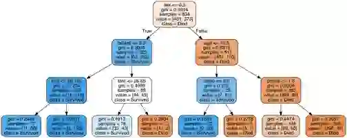
Our depth-10 decision tree is difficult to visualize in a blog post, so to visualize the structure of the decision tree, we created a second tree and limited the tree’s depth to 3. The image below shows the structure of the decision tree, learned by the classifier:
Loading the Redis Predictor
The Redis-ML module provides two commands for working with random forests: ML.FOREST.ADD to create a decision tree within the context of a forest and ML.FOREST.RUN to evaluate a data point using a random forest. The ML.FOREST commands have the following syntax:
ML.FOREST.ADD key tree path ((NUMERIC|CATEGORIC) attr val | LEAF val [STATS]) [...]
ML.FOREST.RUN key sample (CLASSIFICATION|REGRESSION)
Each decision tree in Redis-ML must be loaded using a single ML.FOREST.ADD command. The ML.FOREST.ADD command consists of a Redis key, followed by an integer tree id, followed by node specifications. Node specifications consist of a path, a sequence of . (root), l and r, representing the path to the node in a tree. Interior nodes are splitter or rule nodes and use either the NUMERIC or CATEGORIC keyword to specify the rule type, the attribute to test against and the value of threshold to split. For NUMERIC nodes, the attribute is tested against the threshold and if it is less than or equal to it, the left path is taken; otherwise the right path is taken. For CATEGORIC nodes, the test is equality. Equal values take the left path and unequal values take the right path.
The decision tree algorithm in scikit-learn treats categoric attributes as numeric, so when we represent the tree in Redis, we will only use NUMERIC node types. To load the scikit tree into Redis, we will need to implement a routine that traverses the tree. The following code performs a pre-order traversal of the scikit decision tree to generate a ML.FOREST.ADD command (since we only have a single tree, we generate a simple forest with only a single tree).
# scikit represents decision trees using a set of arrays,
# create references to make the arrays easy to access

the_tree = cl_tree
t_nodes = the_tree.tree_.node_count
t_left = the_tree.tree_.children_left
t_right = the_tree.tree_.children_right
t_feature = the_tree.tree_.feature
t_threshold = the_tree.tree_.threshold
t_value = the_tree.tree_.value
feature_names = df.drop(['survived'], axis=1).columns.values

# create a buffer to build up our command
forrest_cmd = StringIO()
forrest_cmd.write("ML.FOREST.ADD titanic:tree 0 ")

# Traverse the tree starting with the root and a path of “.”
stack = [ (0, ".") ]

while len(stack) > 0:
    node_id, path = stack.pop()

    # splitter node -- must have 2 children (pre-order traversal)
    if (t_left[node_id] != t_right[node_id]):
        stack.append((t_right[node_id], path + "r"))
        stack.append((t_left[node_id], path + "l"))
        cmd = "{} NUMERIC {} {} ".format(path, feature_names[t_feature[node_id]], t_threshold[node_id])
        forrest_cmd.write(cmd)

    else:
        cmd = "{} LEAF {} ".format(path, np.argmax(t_value[node_id]))
        forrest_cmd.write(cmd)

# execute command in Redis
r = redis.StrictRedis('localhost', 6379)
r.execute_command(forrest_cmd.getvalue())
Comparing Results
With the decision tree loaded into Redis, we can create two vectors to compare the predictions of Redis with the predictions from scikit-learn:
# generate a vector of scikit-learn predictors
s_pred = cl_tree.predict(X_test)

# generate a vector of Redis predictions
r_pred = np.full(len(X_test), -1, dtype=int)
for i, x in enumerate(X_test):
    cmd = "ML.FOREST.RUN titanic:tree "

    # iterate over each feature in the test record to build up the
    # feature:value pairs
    for j, x_val in enumerate(x):
        cmd += "{}:{},".format(feature_names[j], x_val)

    cmd = cmd[:-1]
    r_pred[i] = int(r.execute_command(cmd))
To use the ML.FOREST.RUN command, we have to generate a feature vector consisting of a list of comma separated <feature>:<value> pairs. The <feature> portion of the vector is a string feature name that must correspond to the feature names used in the ML.FOREST.ADD command.
Comparing the r_pred and s_pred prediction values against the actual label values:
Y_test: [0 0 0 0 1 0 0 0 1 0 0 0 0 0 1 0 0 0 0 0]
r_pred: [1 0 0 0 1 0 0 0 1 0 0 0 0 0 0 0 0 0 0 0]
s_pred: [1 0 0 0 1 0 0 0 1 0 0 0 0 0 0 0 0 0 0 0]
Redis’ predictions are identical to those of the scikit-learn package, including the misclassification of test items 0 and 14.
An passenger’s chance of survival was strongly correlated to class and gender, so there are several surprising cases of individuals with a high probability of survival who actually perished. Investigating some of these outliers leads to fascinating stories from that fateful voyage. There are many online resources that tell the stories of the Titanic passengers and crew, showing us the people behind the data. I’d encourage you to investigate some of the misclassified people and learn their stories.
In the next and final post we’ll tie everything together and wrap up this introduction to Redis-ML. In the meantime, if you have any questions about this or previous posts, please connect with me (@tague) on Twitter.