Unlocking Time-Series Data with Redis
Learn more


Broadly speaking, there are two types of investors in the world. Fundamental investors look at the fundamental metrics, such as a company’s business model, revenues, earnings, cashflows, current valuation, risks, and growth prospects, when deciding whether to invest in a company. Warren Buffett became famous and one of the world’s richest men by finding undervalued companies through his fundamental research.
On the other hand, technical investors pay very little or no attention to the company’s fundamentals, instead focusing their attention on deriving buy, sell, and hold signals from hundreds of technical indicators. These technical investors trade on a daily, weekly, or monthly basis.
I am not here to argue for or against either of these investing styles. But both fundamental and technical investors study, analyze, and make decisions based on hundreds, if not thousands, of data sources.
Fundamental investors study balance sheets, income statements, cash flow statements, demographic trends, thematic trends, and social trends across thousands of companies and hundreds of industries around the globe. They build financial models or analytics on top of that data to better understand the trajectory of companies and the growth prospects of companies.
Technical investors look at hundreds of technical indicators on an hourly or a daily basis to derive investing signals. Investors who rely on technical indicators have to deal with a vast array of data across multiple time frames to build their trading strategies. They may need to query a vast number of indicators and require virtually instant answers. They may need to quickly adapt their algorithms and trading strategies to fast-changing markets. Redis Enterprise can address all these challenges.
Recently, I wrote about why Redis Enterprise is an essential tool for the financial industry. In this blog post, I will show how RedisTimeSeries can be used to store, aggregate, and query stock prices and technical indicators. The principles I will outline can also be used to store and query financial information from companies or any other time-series data used by fundamental investors.
The RedisTimeSeries module can ingest and query millions of events, samples, and pricing data. RedisTimeSeries is best suited for storing related pairs of times and values to help spot trends in use cases ranging from IoT to healthcare to finance. RedisTimeSeries offers aggregations such as average, sum, minimum, maximum, standard deviation, range, etc. to help you easily analyze data and make decisions.
In this post I am going to illustrate a model for using RedisTimeSeries to store stock prices and technical indicators. I will cover the creation of various time series for prices and indicators, show how to create aggregations on top of the raw time series, and demonstrate how easily bulk time series can be ingested and queried using various RedisTimeSeries commands. I have also provided sample code in Python that you can use as a starting point for your own use case.
Rightly or wrongly, many people consider the Dow Jones Industrial Average (DJIA) the bellwether for the U.S. economy. I wish to track a technical indicator of all the 30 stocks in the DJIA along with the price and trading volume of the stocks. I kick things off by tracking the stock prices of Dow-component Goldman Sachs and one of the technical indicators for that stock. One of my favorite technical indicators is the Relative Strength Index (RSI). RSI is a momentum indicator used to measure a stock that may be in overbought or oversold territory. When the RSI moves near or below 30, a stock may be considered oversold and may present a buying opportunity. Likewise, when the RSI moves above 70, it may be entering overbought territory and signaling a good time to sell.
Relative Strength Index for Goldman Sachs Group
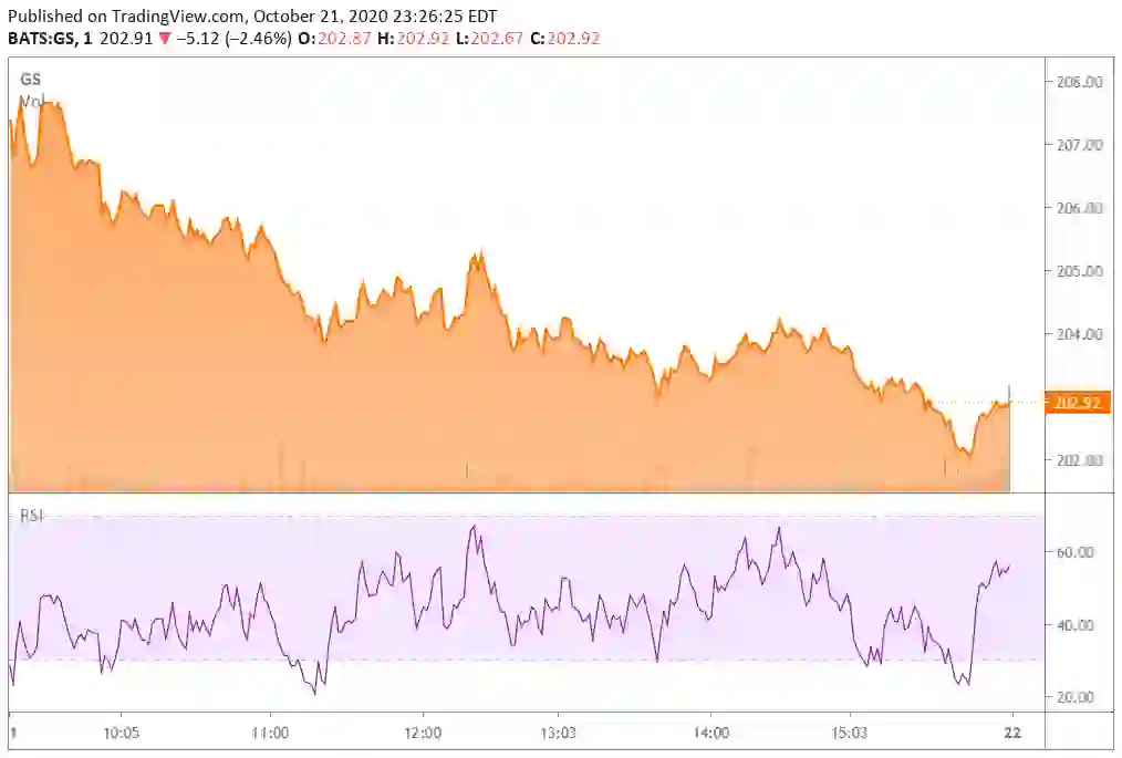
During trading hours, the RSI, just like any other technical indicator, varies as trades are executed based on demand and supply of Goldman Sachs’ shares. We can use the RedisTimeSeries module to help answer a number of key questions:
We can use RedisTimeSeries queries to programmatically identify the minimum and maximum RSI values and stock prices during a designated time period. For example, what if I wanted to find the minimum and maximum RSI numbers during each 15-minute period of the trading day? When the RSI is at or near 30, I may want to generate an alert, place a trade, or kickoff another complex trading workflow to analyze other technical indicators before buying or selling. Anything you wish to do can be easily modeled in a RedisTimeSeries database.
The easiest way to get hands-on experience with RedisTimeSeries is to run the Docker image for RedisTimeSeries.
Execute the following command to pull and run the Docker image:
docker run -p 6379:6379 -it --rm redis/redistimeseries
The Redis team made a deliberate design decision for the RedisTimeSeries module to hold a single metric in each time series. This simplicity in the data model makes the insertion and retrieval of data super fast. You can add new time series as needed without worrying about breaking your existing application. That means you can add new data sources with ease without worrying about breaking the database schema or your application.
Once you have the RedisTimeSeries container up and running you can connect to the server (make sure you have the right IP address or hostname) using Python as follows:
from redistimeseries.client import Client
rts = Client(host='127.0.0.1', port=6379)
With the design principle of holding a single metric in each time series, we can store the intraday stock price and RSI for each of DJIA stock in its own time series. Below, I have created a time series for the Goldman Sachs Group, Inc. (NYSE: GS). I have named the intraday RSI for Goldman Sachs ‘DAILYRSI:GS’ and I have applied various labels to each time series—labeling a time series lets you query across all keys using a label.
rts.create('DAILYRSI:GS',
            labels={ 'SYMBOL': 'GS'
                   , 'DESC':'RELATIVE_STRENGTH_INDEX'
                   , 'INDEX' :'DJIA'
                   , 'TIMEFRAME': '1_DAY'
                   , 'INDICATOR':'RSI'
                   , 'COMPANYNAME': 'GOLDMAN_SACHS_GROUP'})
Here, I have created a time series for Goldman Sachs’ intraday stock prices called ‘INTRADAYPRICES:GS’:
rts.create('INTRADAYPRICES:GS',
            labels={ 'SYMBOL': 'GS'
                   , 'DESC':'SHARE_PRICE'
                   , 'INDEX' :'DJIA'
                   , 'PRICETYPE':'INTRADAY'
                   , 'COMPANYNAME': 'GOLDMAN_SACHS_GROUP'})
Next, I created various aggregations on the RSI data within certain 15-minute timeframes. (We could have created aggregations at longer or shorter time frames to suit our trading needs.) These aggregations will let us look at first, last, min, max, and range values for RSI. To create an aggregation, we first create a time series to store the aggregation and then create a rule to populate the time series with the aggregated value. In this case, we created a time series called ‘DAILYRSI15MINRNG:GS’ to store the range for RSI within a 15-minute time period. The ‘createrule’ applies a range function on the raw data (‘DAILYRSI:GS’) during each 15-minute time frame and aggregates that into ‘DAILYRSI15MINRNG:GS’.
rts.create('DAILYRSI15MINRNG:GS',
            labels={ 'SYMBOL': 'GS'
                   , 'DESC':'RELATIVE_STRENGTH_INDEX'
                   , 'INDEX' :'DJIA'
                   , 'TIMEFRAME': '15_MINUTES'
                   , 'AGGREGATION': 'RANGE'
                   , 'INDICATOR':'RSI'
                   , 'COMPANYNAME': 'GOLDMAN_SACHS_GROUP'})
rts.createrule('DAILYRSI:GS', 'DAILYRSI15MINRNG:GS', 'range', 900)
Here, I created a couple of rules to calculate the range and standard deviation for Goldman Sachs’ stock price during each 15-minute interval during the trading day:
rts.create('INTRADAYPRICES15MINRNG:GS'
          , labels={ 'SYMBOL': 'GS'
                   , 'DESC':'SHARE_PRICE'
                   , 'INDEX' :'DJIA'
                   , 'PRICETYPE':'RANGE'
                   , 'AGGREGATION': 'RANGE'
                   , 'DURATION':'15_MINUTES'
                   , 'COMPANYNAME': 'GOLDMAN_SACHS_GROUP'})

rts.createrule('INTRADAYPRICES:GS’
              ,'INTRADAYPRICES15MINRNG:GS'
              ,'range', 900)

rts.create('INTRADAYPRICES15MINSTDP:GS'
          , labels={ 'SYMBOL': 'GS'
                   , 'DESC':'SHARE_PRICE'
                   , 'INDEX' :'DJIA'
                   , 'PRICETYPE':'STDDEV'
                   , 'AGGREGATION': 'STDDEV'
                   , 'DURATION':'15_MINUTES'
                   , 'COMPANYNAME': 'GOLDMAN_SACHS_GROUP'})

rts.createrule( 'INTRADAYPRICES:GS'
              , 'INTRADAYPRICES15MINSTDP:GS'
              , 'std.p', 900)
You can create time series for all 30 stocks in the Dow Jones Industrial Average (DJIA) in a similar fashion.
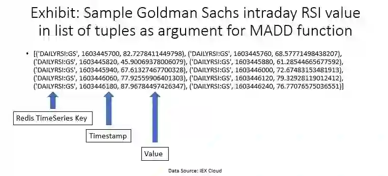
There are two ways to ingest data into the RedisTimeSeries. The TS.ADD command allows you to add each stock price or technical indicator to a time series. But because data from the financial market is produced almost continuously and you need to add multiple samples to RedisTimeSeries, it’s better to use the TS.MADD method. The MADD function takes a list of tuples as an argument. Each tuple takes the name of the time-series key, the timestamp, and the value:
You can use the following Python command to insert data into a time-series key:
rts.madd(<RSIIndicatorList>)
As with most things in RedisTimeSeries, it’s easy to query the database. Range and standard deviation for a stock price or a technical indicator is an indication of volatility. The following query would let you see the price range and standard deviation for the Goldman Sachs stock price within every 15-minute interval:
rts.range( 'INTRADAYPRICES15MINRNG:GS'
         , from_time = 1603704600
         , to_time   = 1603713600)
This query of the range aggregation gives you the following result set:
[(1603704600, 1.75999999999999), (1603705500, 0.775000000000006), (1603706400, 0.730000000000018), (1603707300, 0.449999999999989), (1603708200, 0.370000000000005), (1603709100, 1.01000000000002), (1603710000, 0.490000000000009), (1603710900, 0.89500000000001), (1603711800, 0.629999999999995), (1603712700, 0.490000000000009), (1603713600, 0.27000000000001)]
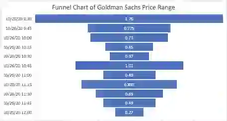
As this query result shows, at the start of the trading day at 9:30 a.m. on October 26, 2020 ET (integer timestamp = 1603704600) the Goldman Sachs stock was volatile, trading with a range of $1.75. Now compare this to the next 15 minutes, starting at 9:45 a.m. on October 26, (integer timestamp = 1603705500), where the volatility dropped with the range of $0.77. The range of prices for Goldman Sachs stock continued to drop in the subsequent 15-minute intervals and the volatility never returned to the levels reached during the opening 15-minute interval.
This data from RedisTimeSeries can be easily visualized in dashboards and charts. The charts below show Goldman Sachs’ price range in 15-minute intervals:
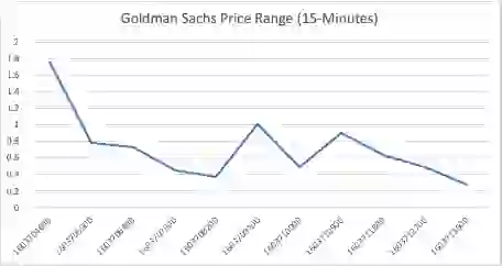
The chart below shows the same data in a line chart format, indicating that the price range in which Goldman Sachs trades becomes much tighter as time progresses through the day (this chart shows integer timestamps on the x-axis):
You can do a similar query with another measure of volatility—standard deviation—as the aggregation function:
rts.range( 'INTRADAYPRICES15MINSTDP:GS'
         , from_time = 1603704600
         , to_time   = 1603713600)
[(1603704600, 0.54657783830434), (1603705500, 0.23201149395202), (1603706400, 0.196072381345986), (1603707300, 0.160267138157647), (1603708200, 0.116990621700049), (1603709100, 0.28043101744222), (1603710000, 0.144379900126934), (1603710900, 0.327611558618967), (1603711800, 0.163118915546951), (1603712700, 0.151417199675549), (1603713600, 0.0963889432843203)]
This opens up many intriguing possibilities. Say you wanted to know the price of Goldman Sachs’ stock when the intraday RSI value is between 30 and 40. You can query the time series for RSI and the time series of the stock prices to identify profitable entry points for a trade.
Here, I am querying the RSI value for Goldman Sachs at a time frame between 1605260100 (9:35 a.m. ET on November 13, 2020) and 1605260940 (9:49 a.m. ET on that day).
dailyGSRSIValue = rts.range( 'DAILYRSI:GS'
                            , from_time = 1605260100
                            , to_time   = 1605260940)
The query finds that the RSI value was 34.2996427544861 at 1605260820 (9:47 a.m. ET).
[(1605260100, 75.0305441024708), (1605260160, 81.6673948350152), (1605260220, 83.8852225932517), (1605260280, 85.9469082344746), (1605260340, 94.3803586011592), (1605260400, 92.2412262502652), (1605260460, 85.6867329371465), (1605260520, 87.9557361513823), (1605260580, 89.9407873066781), (1605260640, 57.1512452602676), (1605260700, 50.5638232111769), (1605260760, 35.2804436894564), (1605260820, 34.2996427544861), (1605260880, 54.5486275202972), (1605260940, 64.7593307385219)]
Now I can query the Goldman Sachs’ intraday prices for the same interval as the one used for the RSI query, or change the query programmatically to reflect when the RSI value was at 34.29. Here’s an example using the same time frame as the RSI query.
dailyGSPrice = rts.range( 'INTRADAYPRICES:GS'
                         , from_time = 1605260100
                         , to_time   = 1605260940)
The query returns Goldman Sachs’ stock prices for the specified range: At 1605260820 (9:47 a.m. ET on November 13, 2020) the price was $217.18.
[(1605260100, 216.57), (1605260160, 216.73), (1605260220, 217.08), (1605260280, 217.17), (1605260340, 217.87), (1605260400, 218.05), (1605260460, 217.91), (1605260520, 218.0), (1605260580, 218.11), (1605260640, 218.02), (1605260700, 217.72), (1605260760, 217.22), (1605260820, 217.18), (1605260880, 217.46), (1605260940, 217.61)]
RedisTimeSeries offers a powerful way to query across multiple time series at once. The TS.MGET command lets you query across multiple time series using filters. We have already created various time series and attached labels to them. Now those labels can act as filters to query across the time series.
The following Python code applies two filters based on a couple of labels: “DESC” and “TIMEFRAME”. The parameter “with_labels=False” allows the result set to be returned without the labels for each value:
allRSIValues = rts.mget(filters=['DESC=RELATIVE_STRENGTH_INDEX','TIMEFRAME=1_DAY'], with_labels=False)
This query would present a result similar to the one shown here, which returns the last RSI values across a number of stocks:
[{'DAILYRSI:BA': [{}, 1605261060, 62.2048922111768]}, {'DAILYRSI:CAT': [{}, 1605261060, 68.3834400302296]}, {'DAILYRSI:CRM': [{}, 1605261060, 59.2107333830133]}, {'DAILYRSI:CSCO': [{}, 1605261060, 52.7011052724688]}, {'DAILYRSI:CVX': [{}, 1605261060, 62.9890368832232]}, {'DAILYRSI:DOW': [{}, 1605261060, 73.597680480764]}, {'DAILYRSI:GS': [{}, 1605283140, 41.182852552541]}, {'DAILYRSI:IBM': [{}, 1605261060, 65.3742140862697]}, {'DAILYRSI:JPM': [{}, 1605261060, 77.7760292843745]}, {'DAILYRSI:KO': [{}, 1605261060, 26.8638381005608]}, {'DAILYRSI:MMM': [{}, 1605261060, 65.7852833683174]}, {'DAILYRSI:MRK': [{}, 1605261060, 38.9991886598036]}, {'DAILYRSI:UNH': [{}, 1605261060, 74.2672428885775]}, {'DAILYRSI:VZ': [{}, 1605261060, 33.177554436462]}, {'DAILYRSI:WBA': [{}, 1605261060, 47.3877762365391]}]
If I had set “with_labels=True”, then the result would have included all the labels on each of the time series, as shown here:
[{'DAILYRSI:BA': [{'SYMBOL': 'BA', 'DESC': 'RELATIVE_STRENGTH_INDEX', 'INDEX': 'DJIA', 'TIMEFRAME': '1_DAY', 'INDICATOR': 'RSI', 'COMPANYNAME': 'BOEING'}, 1605261060, 62.2048922111768]}, {'DAILYRSI:CAT': [{'SYMBOL': 'CAT', 'DESC': 'RELATIVE_STRENGTH_INDEX', 'INDEX': 'DJIA', 'TIMEFRAME': '1_DAY', 'INDICATOR': 'RSI', 'COMPANYNAME': 'CATERPILLAR'}, 1605261060, 68.3834400302296]}, {'DAILYRSI:CRM': [{'SYMBOL': 'CRM', 'DESC': 'RELATIVE_STRENGTH_INDEX', 'INDEX': 'DJIA', 'TIMEFRAME': '1_DAY', 'INDICATOR': 'RSI', 'COMPANYNAME': 'SALESFORCE'}, 1605261060, 59.2107333830133]}]
This blog post has illustrated some of RedisTimeSeries’ many commands to flexibly build a financial application that is dependent on time-series data. Stock traders, for example, need to be able to make high-stakes decisions in real time based on dozens of variables. RedisTimeSeries is schemaless, which means that you can load data without defining schema, add new fields on the fly, or change your data model should your business circumstances change. Its real-time performance and simple developer experience makes it fun to work with time-series data!
You can find the sample code for this blog post on GitHub here. And you can learn more about RedisTimeSeries here.